Tutorials and example datasets
MotilA provides Jupyter notebooks and Python scripts that demonstrate the complete analysis workflow. Also, an example dataset is publicly available on Zenodo. These resources enable users to validate their installation, understand the processing steps and reproduce the results shown in the associated manuscript.
Example dataset
A curated example dataset is available on Zenodo: Gockel & Nieves-Rivera & Musacchio et al. (2025), doi: 10.5281/zenodo.15061566; the dataset is based on Gockel & Nieves-Rivera et al., 2026.
The dataset contains:
a representative 5D time-lapse image stack,
a corresponding
metadata.xlsfile with projection center settings, anda ready-to-use project folder structure compatible with MotilA.
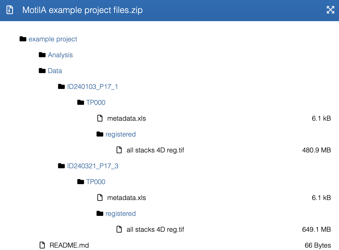
Contents of the Zenodo example dataset, including the required project-folder
structure for batch processing. The dataset mirrors the directory layout
expected by MotilA, with ID folders, project_tag subfolders,
registered image stacks, and an accompanying metadata.xls file.
After downloading, place the dataset into the example_project directory of
your MotilA working directory (i.e., the folder, where you run the scripts from).
An example of the expected folder structure can also be found in the repository.
Running MotilA directly on this dataset allows users to verify that the pipeline is functioning correctly and produces meaningful motility metrics.
We also provide a smaller “cutout” version of the example dataset for quick testing and demonstration purposes: Musacchio (2025), doi: 10.5281/zenodo.17803977.
If you use one of the provided datasets for any purpose beyond the example tutorials, please cite both the dataset record (Gockel & Nieves-Rivera & Musacchio et al., 2025, doi: 10.5281/zenodo.15061566 / Musacchio, 2025, doi: 10.5281/zenodo.17803977) and Gockel & Nieves-Rivera et al., 2026.
Tutorial notebooks
MotilA includes Jupyter notebooks that illustrate the core processing steps on the example data:
single_file_run.ipynb Demonstrates the complete workflow for processing a single image stack.
batch_run.ipynb Shows how to process multiple datasets stored in a structured project folder.
These notebooks guide users through image loading, optional preprocessing, motility computation and inspection of intermediate and final results. They serve as the most accessible introduction to the pipeline.
Example Python scripts
Equivalent Python scripts are provided for users who prefer script-based workflows or who want to integrate MotilA into automated analysis pipelines:
These scripts mirror the behavior of the tutorial notebooks and can be adapted for larger projects or command-line environments.
Reproducing manuscript figures
The figures shown in the associated manuscript were generated using a dedicated script that applies MotilA to a specific subset of the example dataset:
The subset used for figure generation is located at:
example_project/Data/ID240103_P17_1_cutout/TP000
The script contains all parameter settings used during analysis and can be used to reproduce the manuscript figures exactly.
Additional example datasets
The repository may include additional reduced datasets, project templates or
folder structures intended to help users set up their own analyses. These
resources are located in the example_project directory and follow the same
format expected by the batch processing routines of MotilA. They can be used as
templates for structuring new experimental datasets.
Example usage
The following examples illustrate how to use MotilA in practice, starting from a registered time-lapse stack and proceeding through single-file processing, batch processing and batch-level result collection.
MotilA uses OMIO to read TIFF/OME-TIFF, CZI, Thorlabs RAW and LSM files and
normalizes them to TZCYX, with T denoting time, Z depth, C channels and X/Y the
spatial dimensions. See the data requirements for
details on axis order, multi-channel handling and the optional legacy TIFF axis
correction function tiff_axes_check_and_correct.
Single-file processing
Import MotilA and initialize logging:
import motila as mt
from pathlib import Path

# verify installation
mt.hello_world()

# initialize logger
log = mt.logger_object()
Parameter selection
Before calling motila.process_stack(), you should choose parameter values
that match your imaging protocol and data quality. A complete description of
all arguments is given in the parameter documentation.
Below is a practical guide for the most important groups of parameters.
Projection parameters
The parameters projection_center and projection_layers control the
subvolume that is projected:
For sparsely distributed microglia, a symmetric window of approximately 7 to 13 z-layers centered on the cell of interest is usually sufficient.
For densely packed microglia, it is often advisable to process several subvolumes with different projection centers in order to reduce overlap of processes in the projection.
Ensure that the chosen subvolume fits inside the stack dimensions. MotilA performs a sanity check and will adjust the subvolume if it exceeds the image bounds, but this may reduce the effective number of projected slices.
Registration parameters
If there is visible motion across time, registration should be enabled:
regStack3d=Trueif there is intra-stack motion within the 3D volume at each time point (for example breathing or slow drift along z).regStack2d=Trueif residual lateral drift remains after 3D registration or if only projections are available.
The parameter template_mode controls how the 3D registration template is
computed. A typical choice is "mean" (default), while "median" may be
more robust for occasional outlier frames. The parameter
max_xy_shift_correction limits the allowed x/y shift and can be used to
avoid overcorrection if rare frames contain large artefacts.
Histogram equalization and matching
Two complementary mechanisms adjust contrast and compensate for bleaching:
hist_equalization=Trueapplies CLAHE within each stack. This is recommended for low-contrast images or uneven illumination. Start with a clip limit around0.05and adjust only if necessary.hist_match=Truenormalizes the intensity distribution across time. Select a representative time point ashistogram_ref_stack(for example a mid-sequence frame without strong artefacts).
Histogram equalization improves local contrast but can amplify noise if the clip limit is chosen too high. Histogram matching makes the time series more comparable but will transfer noise patterns from the reference stack if that stack is of poor quality.
Filtering parameters
Filtering reduces noise and small artefacts before segmentation:
median_filter_slicesandmedian_filter_projectionsapply median filters either slice-wise or on the 2D projections. Use"square"with odd kernel sizes (such as 3 or 5) for general noise reduction. Use"circular"if you aim to emulate ImageJ or Fiji.gaussian_sigma_projapplies a Gaussian blur on the projection. A value around 1 to 2 pixels is a reasonable starting point. Use 0 to disable Gaussian smoothing.
Median filtering is useful when salt-and-pepper noise or small speckles dominate. Gaussian smoothing is useful for reducing high-frequency noise in otherwise smooth structures.
Spectral unmixing parameters
For two-channel recordings with bleed-through from the second channel into the microglia channel, enable spectral unmixing:
Set
spectral_unmixing=Trueif there is visible contamination of the microglia channel by the second channel.spectral_unmixing_amplifyercan be used to slightly amplify the microglia channel before subtraction, for example values between 1 and 2.spectral_unmixing_median_filter_windowcontrols smoothing of the second channel before subtraction. Typical values are 1 (off), 3 or 5.
Spectral unmixing is most effective when the bleed-through is relatively uniform and the second channel has good signal-to-noise ratio. If the overlap is highly non-linear or dominated by noise, unmixing may not improve the result.
Tip
The spectral unmixing method implemented in MotilA is rather simple: It just subtracts the second channel from the microglia channel after optional smoothing and amplification. For a more sophisticated approach, consider using dedicated spectral unmixing software or plugins, for example in ImageJ/Fiji or Spectral Unmixing) before running MotilA.
Example parameter values
Below is a minimal, representative parameter configuration taken from the
official tutorial script single_file_run.py. These values demonstrate how
MotilA is typically used on the included example dataset. They are meant as a
practical starting point and can be adapted to your own data.
# dataset identification
Current_ID = "ID240103_P17_1"
group      = "blinded"

# input file
DATA_Path  = "../example_project/Data/ID240103_P17_1/TP000/registered/"
IMG_File   = "all stacks 4D reg.tif"
fname      = Path(DATA_Path).joinpath(IMG_File)

# projection settings
projection_layers = 44
projection_center = 23

# output path
RESULTS_foldername = f"../motility_analysis/projection_center_{projection_center}/"
RESULTS_Path = Path(DATA_Path).joinpath(RESULTS_foldername)
mt.check_folder_exist_create(RESULTS_Path)

# thresholding
threshold_method = "otsu"
blob_pixel_threshold = 100
compare_all_threshold_methods = True

# image enhancement
hist_equalization = True
hist_equalization_clip_limit = 0.05
hist_equalization_kernel_size = None
hist_match = True
histogram_ref_stack = 0

# filtering
median_filter_slices = "circular"
median_filter_window_slices = 1.55
median_filter_projections = "circular"
median_filter_window_projections = 1.55
gaussian_sigma_proj = 1.0

# channels
two_channel = True
MG_channel = 0
N_channel  = 1

# registration
regStack3d = True
regStack2d = False
template_mode = "max"
max_xy_shift_correction = 100

# spectral unmixing
spectral_unmixing = True
spectral_unmixing_amplifyer = 1
spectral_unmixing_median_filter_window = 3

# book-keeping
clear_previous_results = True
log = mt.logger_object()
Calling the processing function
After defining the necessary parameters, run the pipeline:
mt.process_stack(
  fname=fname,
  MG_channel                   = MG_channel,
  N_channel                    = N_channel,
  two_channel                  = two_channel,
  projection_layers            = projection_layers,
  projection_center            = projection_center,
  histogram_ref_stack          = histogram_ref_stack,
  log                          = log,
  blob_pixel_threshold         = blob_pixel_threshold,
  regStack2d                   = regStack2d,
  regStack3d                   = regStack3d,
  template_mode                = template_mode,
  spectral_unmixing            = spectral_unmixing,
  hist_equalization            = hist_equalization,
  hist_equalization_clip_limit = hist_equalization_clip_limit,
  hist_equalization_kernel_size= hist_equalization_kernel_size,
  hist_match                   = hist_match,
  RESULTS_Path                 = RESULTS_Path,
  ID                           = Current_ID,
  group                        = group,
  threshold_method             = threshold_method,
  compare_all_threshold_methods= compare_all_threshold_methods,
  gaussian_sigma_proj          = gaussian_sigma_proj,
  spectral_unmixing_amplifyer  = spectral_unmixing_amplifyer,
  median_filter_slices         = median_filter_slices,
  median_filter_window_slices  = median_filter_window_slices,
  median_filter_projections    = median_filter_projections,
  median_filter_window_projections= median_filter_window_projections,
  clear_previous_results       = clear_previous_results,
  spectral_unmixing_median_filter_window= spectral_unmixing_median_filter_window,
  debug_output                 = debug_output,
  stats_plots                  = stats_plots)
For a compact overview of all parameters and their allowed values, see the parameter reference.
Batch processing
Batch processing uses the same parameters but operates on multiple datasets organized in a project folder. In addition, the following parameters control which datasets are processed and where the results are written:
project_rootspecifies the root directory containing all subject folders.subject_idsselects exact subjects, orsubject_prefixdiscovers matching subjects automatically.tag_folder_levelsdescribes the flexible folder levels below each subject.image_patternsselects supported image files by glob pattern;Noneuses MotilA’s TIFF/OME-TIFF, CZI, LSM and RAW defaults.exclude_name_containsfilters unwanted files or folders such as previews.results_folder_namedefines where MotilA results are stored.skip_processedskips files whose expected output already exists and records them as already processed in the run report.metadata_file(for example"metadata.xls") optionally overrides parameters such as channel indices or projection centers on a per-dataset basis.
A detailed description of the expected folder structure and metadata handling is given in the parameter documentation.
Example batch configuration
The following parameter set is taken from the tutorial script
batch_run.py and demonstrates how to batch-process the included example
datasets from the Zenodo record:
PROJECT_ROOT = "../example_project/Data/"

subject_ids = ["ID240103_P17_1", "ID240321_P17_3"]
subject_prefix = "ID"

tag_folder_levels = [
    ("TP000",),
    ("registered",)]

image_patterns = None
# image_patterns = ("*reg*.ome.tif", "*reg*.tif")
exclude_name_contains = ("Preview",)

# projection settings
projection_layers = 44
projection_center = 23

# thresholding
threshold_method = "otsu"
blob_pixel_threshold = 100
compare_all_threshold_methods = True

# image enhancement
hist_equalization = True
hist_equalization_clip_limit = 0.1
hist_equalization_kernel_size = (128, 128)
hist_match = True
histogram_ref_stack = 0

# filtering
median_filter_slices = "circular"
median_filter_window_slices = 1.55
median_filter_projections = "circular"
median_filter_window_projections = 1.55
gaussian_sigma_proj = 1.0

# channels
two_channel = True
MG_channel = 0
N_channel = 1

# registration
regStack3d = True
regStack2d = False
template_mode = "max"
max_xy_shift_correction = 100

# spectral unmixing
spectral_unmixing = True
spectral_unmixing_amplifyer = 1
spectral_unmixing_median_filter_window = 3

# housekeeping
log = mt.logger_object()

processing_options = {
    "MG_channel": MG_channel,
    "N_channel": N_channel,
    "two_channel": two_channel,
    "projection_center": projection_center,
    "projection_layers": projection_layers,
    "histogram_ref_stack": histogram_ref_stack,
    "log": log,
    "blob_pixel_threshold": blob_pixel_threshold,
    "regStack2d": regStack2d,
    "regStack3d": regStack3d,
    "template_mode": template_mode,
    "spectral_unmixing": spectral_unmixing,
    "hist_equalization": hist_equalization,
    "hist_equalization_clip_limit": hist_equalization_clip_limit,
    "hist_equalization_kernel_size": hist_equalization_kernel_size,
    "hist_match": hist_match,
    "max_xy_shift_correction": max_xy_shift_correction,
    "threshold_method": threshold_method,
    "compare_all_threshold_methods": compare_all_threshold_methods,
    "gaussian_sigma_proj": gaussian_sigma_proj,
    "spectral_unmixing_amplifyer": spectral_unmixing_amplifyer,
    "median_filter_slices": median_filter_slices,
    "median_filter_window_slices": median_filter_window_slices,
    "median_filter_projections": median_filter_projections,
    "median_filter_window_projections": median_filter_window_projections,
    "clear_previous_results": False,
    "spectral_unmixing_median_filter_window": spectral_unmixing_median_filter_window,
    "debug_output": debug_output,
    "stats_plots": stats_plots}
These values provide a realistic starting point and can be adapted to new projects by changing the paths, subject selection, folder-tag levels and, if necessary, the preprocessing and segmentation settings.
The batch-processing call is:
result = mt.batch_process_stacks(
    project_root           = PROJECT_ROOT,
    subject_ids            = subject_ids,
    subject_prefix         = subject_prefix,
    tag_folder_levels      = tag_folder_levels,
    image_patterns         = image_patterns,
    exclude_name_contains  = exclude_name_contains,
    skip_processed         = True,
    results_folder_name    = "motility_analysis",
    organize_by_image      = True,
    metadata_file          = "metadata.xls",
    load_options           = {"preflight": False},
    processing_options     = processing_options,
    save_options           = {"validate_outputs": True},
    log                    = log,
    verbose                = True)
result contains the discovered, processed, skipped and failed files. MotilA
also updates motila_batch_run_report.txt in PROJECT_ROOT after each run.
If errors occur, a timestamped motila_batch_error_report_*.txt is written in
the project root and shorter per-file reports are written next to affected image
files.
Batch collection
After batch processing, the results from multiple datasets can be aggregated for cohort-level analysis. The key parameters are:
project_rootpointing to the same project root as in batch processing.subject_idsorsubject_prefixselecting the same subjects.tag_folder_levels,image_patternsandexclude_name_containsusing the same discovery settings asbatch_process_stacks.results_folder_namespecifying the folder where MotilA wrote the per-dataset results.organize_by_imagematching the processing run.RESULTS_Pathdefining the output directory for the aggregated cohort tables.
Example batch collection configuration
The following configuration mirrors the settings used in the tutorial script
batch_run.py for collecting results from the example_project:
PROJECT_ROOT = "../example_project/Data/"
RESULTS_Path = "../example_project/Analysis/MG_motility/"

subject_ids = ["ID240103_P17_1", "ID240321_P17_3"]
tag_folder_levels = [
    ("TP000",),
    ("registered",)]

log = mt.logger_object()
Aggregate results across multiple datasets with:
collection_result = mt.batch_collect(
    project_root           = PROJECT_ROOT,
    subject_ids            = subject_ids,
    subject_prefix         = "ID",
    tag_folder_levels      = tag_folder_levels,
    image_patterns         = None,
    exclude_name_contains  = ("Preview",),
    results_folder_name    = "motility_analysis",
    organize_by_image      = True,
    RESULTS_Path           = RESULTS_Path,
    log                    = log,
    verbose                = True)
Assessing your results
Single-file results include TIFF and PDF files for each processing step as well
as an Excel file motility.xlsx containing:
gained pixels (G),
lost pixels (L),
stable pixels (S),
turnover rate (TOR).
Additional Excel files summarize brightness metrics and cell pixel areas. The brightness measures allow you to assess bleaching and signal stability over time. The cell pixel area is expected to remain relatively stable if the microglial cells do not leave the field of view or disappear.
Excel remains MotilA’s default table format for backward compatibility. If you
also need plain-text outputs, set table_export_formats=("excel", "csv",
"yaml") in motila.process_stack(), motila.batch_process_stacks()
or motila.batch_collect(). MotilA then writes matching .csv and
.yaml sidecar files next to the default .xlsx tables.
Batch processing generates cohort-level summary files:
all_motility.xlsxall_brightness.xlsxall_cell_pixel_area.xlsxaverage_motility.xlsx
These files can be used to compare experimental groups, quantify effects of manipulations and create summary plots for publication.